Tables with summary rows in gt
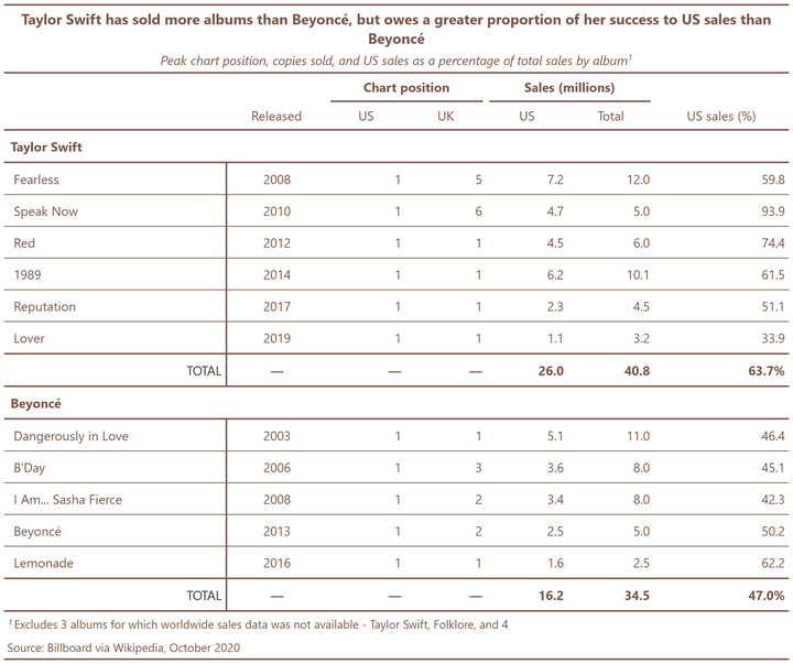
This post focuses on ways to customize summary rows in gt tables, to create the summary table shown here (based on the Tidy Tuesday Taylor Swift and Beyoncé data).
Setup
First, let’s load packages and read in the data (as manipulated in a previous post):
#load packages
library(tidyverse)
library(gt) # for summary tables

#load data
albums <- read.csv('https://raw.githubusercontent.com/lynleyaldridge/tidytuesday/main/2020/2020-week40/data/albums.csv')
Adding summary rows with more complex calculations
One thing I’ve learned in my journey with R so far is that ‘finishing that off’ with ‘just one more thing’ can involve a considerable amount of work when you’re teaching yourself as you go. I was keen, however, to create a table summarizing total US and worldwide sales for each artist, and calculating what percentage of each artist’s total sales was represented by US sales. I drew on general guidance for creating summary lines in creating my first gt table on this blog.
Thanks to josep maria porrà for providing an example on stack overflow I was able to modify further to create the below code.
First, we need to create a new data frame calculating US sales as a percentage of total sales for each artist:
albums_grouped <- albums %>%
  drop_na() %>%
  group_by(artist) %>%
  summarise_at(vars(US_sales, WW_sales), sum) %>%
  rowwise() %>%
  mutate(pct_US = US_sales/WW_sales)

albums_grouped
## # A tibble: 2 x 4
## # Rowwise:
##   artist       US_sales WW_sales pct_US
##   <chr>           <dbl>    <dbl>  <dbl>
## 1 Beyoncé          16.2     34.5  0.470
## 2 Taylor Swift     26       40.8  0.637
These will be the values that we pull into the summary rows. Now, let’s make a table based on selected columns from the original albums data frame, dropping albums with missing sales data. Using the gt() function, we can specify desired columns to use as row names and grouping variables (rowname_col = "title, groupname_col = "artist").
In order to create the summary rows, first summarize the US_sales and WW_sales columns, using the sum function and reporting output as TOTAL. Then select the pct_US for the Taylor Swift row in albums_grouped, and retrieve as TOTAL for the Taylor Swift group. Repeat for Beyoncé. The formatter = argument allows formatting numbers as percentages, to specified number of decimal points. Finally, we can use tab_style() to style our group names and summary rows:
gt1 <- albums %>%

  select(title, artist, year, US_chart, UK_chart, US_sales, WW_sales, US_percent) %>%
  drop_na() %>%
  gt(rowname_col = "title", groupname_col = "artist") %>%

    # create summary rows for each group
    summary_rows(groups = TRUE,
                 columns = vars(US_sales, WW_sales),
                 fns = list(TOTAL = "sum"),
                 formatter = fmt_number, decimals = 1) %>%
    summary_rows(groups = "Taylor Swift",
                 columns = vars(US_percent),
                 fns = list(TOTAL = ~
                            albums_grouped %>%
                            filter(artist == "Taylor Swift") %>%
                            select(pct_US) %>%
                            pull()),
                 formatter = fmt_percent, decimals = 1) %>%
    summary_rows(groups = "Beyoncé",
                 columns = vars(US_percent),
                 fns = list(TOTAL = ~
                            albums_grouped %>%
                            filter(artist == "Beyoncé") %>%
                            select(pct_US) %>%
                            pull()),
                 formatter = fmt_percent, decimals = 1) %>%

    # style summary rows and row group titles
    tab_style(style = cell_text(weight = "bold",
                                color = "#795548"),
        locations = list(cells_summary(groups = TRUE),
                          cells_row_groups(groups = TRUE)))

gt1
| year | US_chart | UK_chart | US_sales | WW_sales | US_percent | |
|---|---|---|---|---|---|---|
| Taylor Swift | ||||||
| Fearless | 2008 | 1 | 5 | 7.2 | 12.0 | 59.8 |
| Speak Now | 2010 | 1 | 6 | 4.7 | 5.0 | 93.9 |
| Red | 2012 | 1 | 1 | 4.5 | 6.0 | 74.4 |
| 1989 | 2014 | 1 | 1 | 6.2 | 10.1 | 61.5 |
| Reputation | 2017 | 1 | 1 | 2.3 | 4.5 | 51.1 |
| Lover | 2019 | 1 | 1 | 1.1 | 3.2 | 33.9 |
| TOTAL | — | — | — | 26.0 | 40.8 | 63.7% |
| Beyoncé | ||||||
| Dangerously in Love | 2003 | 1 | 1 | 5.1 | 11.0 | 46.4 |
| B'Day | 2006 | 1 | 3 | 3.6 | 8.0 | 45.1 |
| I Am... Sasha Fierce | 2008 | 1 | 2 | 3.4 | 8.0 | 42.3 |
| Beyoncé | 2013 | 1 | 2 | 2.5 | 5.0 | 50.2 |
| Lemonade | 2016 | 1 | 1 | 1.6 | 2.5 | 62.2 |
| TOTAL | — | — | — | 16.2 | 34.5 | 47.0% |
To finalize this table, we follow the steps outlined in a previous post on gt tables to assign column labels and column spanner headings, set column alignment, cell color and formatting, and give the table a title, subtitle and source note:
gt2 <- gt1 %>%

    cols_label(
      year = "Released",
      US_chart = "US",
      UK_chart = "UK",
      US_sales = "US",
      WW_sales = "Total",
      US_percent = "US sales (%)") %>%

    tab_spanner(label = "Chart position", columns = vars(US_chart,
                                                         UK_chart)) %>%
    tab_spanner(label = "Sales (millions)", columns = vars(US_sales,
                                                            WW_sales)) %>%

    cols_align(align = "right", columns = c("US_chart", "UK_chart",
                                            "US_sales", "WW_sales",
                                            "US_percent")) %>%

    tab_style(style = cell_text(color = "#795548"),
          locations = list(
            cells_column_labels(everything()),
            cells_stub(rows = TRUE),
            cells_body()))%>%

    tab_style(style = cell_text(
      color = "#795548",
      weight = "bold"),
      locations = cells_column_spanners(spanners = vars("Chart position",
                                                      "Sales (millions)")))%>%

    tab_header(
      title = md(
        "**Taylor Swift has sold more albums than Beyoncé, but owes a greater proportion of her success to US sales than Beyoncé**"),
      subtitle = md(
        "*Peak chart position, copies sold, and US sales as a percentage of total sales by album*")) %>%

    tab_source_note(
      source_note = md("<span style = 'color:#795548'>Source: Billboard via Wikipedia, October 2020<br>Excludes 3 albums for which worldwide sales data was not available - Taylor Swift, Folklore, and 4</span>")) %>%

    tab_style(style = cell_text(color = "#795548", size = "large"),
          locations = cells_title(groups = "title")) %>%

    tab_style(style = cell_text(color = "#795548", size = "medium"),
          locations = cells_title(groups = "subtitle"))

gt2
| Taylor Swift has sold more albums than Beyoncé, but owes a greater proportion of her success to US sales than Beyoncé | ||||||
|---|---|---|---|---|---|---|
| Peak chart position, copies sold, and US sales as a percentage of total sales by album | ||||||
| Released | Chart position | Sales (millions) | US sales (%) | |||
| US | UK | US | Total | |||
| Taylor Swift | ||||||
| Fearless | 2008 | 1 | 5 | 7.2 | 12.0 | 59.8 |
| Speak Now | 2010 | 1 | 6 | 4.7 | 5.0 | 93.9 |
| Red | 2012 | 1 | 1 | 4.5 | 6.0 | 74.4 |
| 1989 | 2014 | 1 | 1 | 6.2 | 10.1 | 61.5 |
| Reputation | 2017 | 1 | 1 | 2.3 | 4.5 | 51.1 |
| Lover | 2019 | 1 | 1 | 1.1 | 3.2 | 33.9 |
| TOTAL | — | — | — | 26.0 | 40.8 | 63.7% |
| Beyoncé | ||||||
| Dangerously in Love | 2003 | 1 | 1 | 5.1 | 11.0 | 46.4 |
| B'Day | 2006 | 1 | 3 | 3.6 | 8.0 | 45.1 |
| I Am... Sasha Fierce | 2008 | 1 | 2 | 3.4 | 8.0 | 42.3 |
| Beyoncé | 2013 | 1 | 2 | 2.5 | 5.0 | 50.2 |
| Lemonade | 2016 | 1 | 1 | 1.6 | 2.5 | 62.2 |
| TOTAL | — | — | — | 16.2 | 34.5 | 47.0% |
| Source: Billboard via Wikipedia, October 2020 Excludes 3 albums for which worldwide sales data was not available - Taylor Swift, Folklore, and 4 |
||||||
To save this table as a .png image, use the following code (amending path as desired):
library(here)
gtsave(gt2, here::here("compare-sales.png"))
See my tidytuesday repository for the full code used to generate the image at the top of this post, which includes additional code for footnotes and borders.
Lynley Aldridge
My research interests include social and educational inequality, transitions from education to employment, education, cross-cultural comparative research, migration/mobility, mental health/wellbeing, and Rstats.